Show the code
rest_received <- read_csv("files/Daily_Restaurant_Received_Orders_Data.csv")
rest_sales <- read_csv("files/Daily_Restaurant_Sales_Data.csv")
menu_data <- read_csv("files/Menu_Item_Recipe_Data.csv")
Before jumping right into the coding part, let’s first understand the network flow we are going to work on.
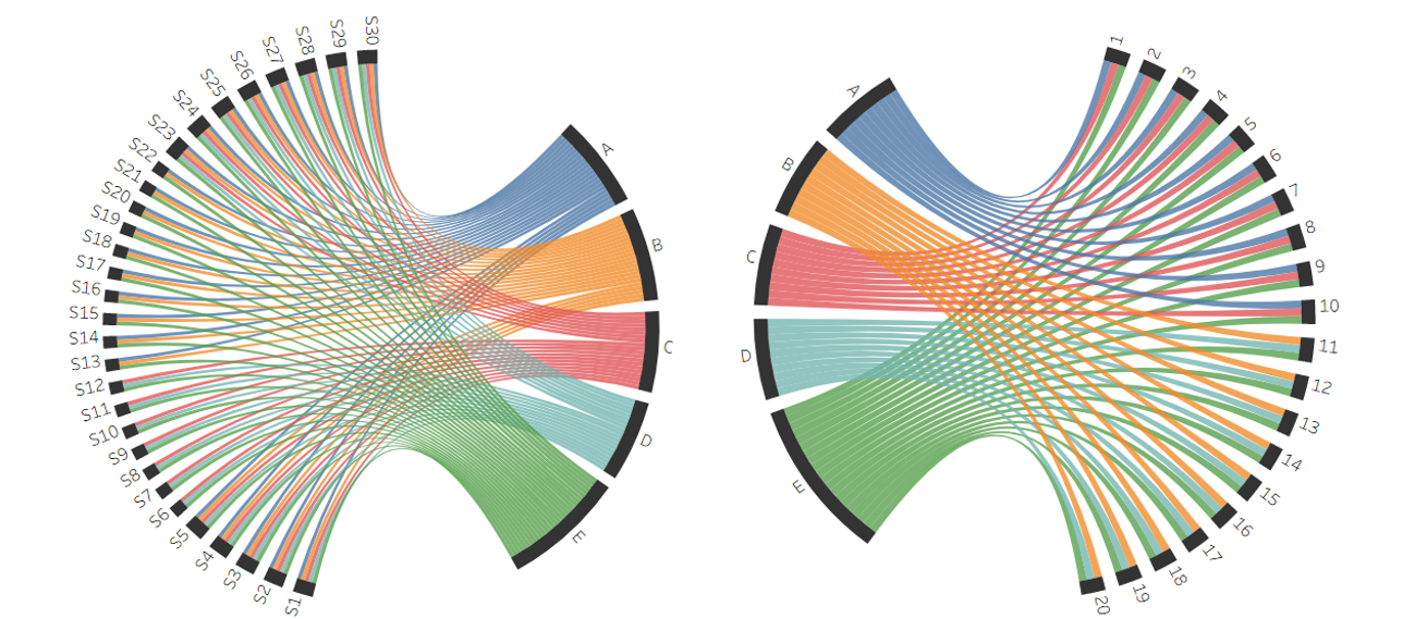
The above visual helps us understand better about the flow of products across the layers in our multi echelon supply chain. It is evident that distribution center E is playing a vital role in the network, as it is the only D.C that handles all kind of products while maintaining a direct relation with all the Suppliers and Restaurants.
rest_received <- read_csv("files/Daily_Restaurant_Received_Orders_Data.csv")
rest_sales <- read_csv("files/Daily_Restaurant_Sales_Data.csv")
menu_data <- read_csv("files/Menu_Item_Recipe_Data.csv")Let us first understand a bit about the datasets.
rest_received# A tibble: 36,600 × 4
Day Restaurant Product_Category Received_Order_Volume
<dbl> <dbl> <chr> <dbl>
1 1 1 Bakery 50
2 1 1 Beverages 178
3 1 1 Dairy 87
4 1 1 Meat 52
5 1 1 Vegetables 167
6 1 2 Bakery 41
7 1 2 Beverages 109
8 1 2 Dairy 63
9 1 2 Meat 43
10 1 2 Vegetables 125
# ℹ 36,590 more rowsrest_sales# A tibble: 51,240 × 4
Day Restaurant Menu_Item Quantity_Sold
<dbl> <dbl> <chr> <dbl>
1 1 1 Burger 65
2 1 1 Coffee 78
3 1 1 Fries 58
4 1 1 Milkshake 61
5 1 1 Pizza 64
6 1 1 Salad 67
7 1 1 Soft Drink 72
8 1 2 Burger 54
9 1 2 Coffee 35
10 1 2 Fries 41
# ℹ 51,230 more rowsmenu_data# A tibble: 35 × 3
Menu_Item Product_Category Percentage_Required
<chr> <chr> <dbl>
1 Burger Meat 50
2 Burger Dairy 11
3 Burger Vegetables 17
4 Burger Beverages 0
5 Burger Bakery 22
6 Pizza Meat 16
7 Pizza Dairy 20
8 Pizza Vegetables 18
9 Pizza Beverages 0
10 Pizza Bakery 46
# ℹ 25 more rowsI assumed that the excess products at each layer along the supply chain are considered perishable at the end of the day. Hence considered wastage.
Let’s pivot the menu_data in order to link it up with sales data.
pivot_menu_data <- menu_data |>
  pivot_wider(names_from = Product_Category, values_from = Percentage_Required, values_fill = list(Percentage_Required = 0))
pivot_menu_data
# A tibble: 7 × 6
Menu_Item Meat Dairy Vegetables Beverages Bakery
<chr> <dbl> <dbl> <dbl> <dbl> <dbl>
1 Burger 50 11 17 0 22
2 Pizza 16 20 18 0 46
3 Salad 0 11 89 0 0
4 Soft Drink 0 0 0 100 0
5 Coffee 0 14 0 86 0
6 Fries 0 0 100 0 0
7 Milkshake 0 60 0 40 0I would now like to convert the items names into raw products names. For this, I would merge the Restautant Sales with pivoted menu data.
merged_data <- rest_sales |>
  left_join(pivot_menu_data, by = "Menu_Item")
merged_data
# A tibble: 51,240 × 9
Day Restaurant Menu_Item Quantity_Sold Meat Dairy Vegetables Beverages
<dbl> <dbl> <chr> <dbl> <dbl> <dbl> <dbl> <dbl>
1 1 1 Burger 65 50 11 17 0
2 1 1 Coffee 78 0 14 0 86
3 1 1 Fries 58 0 0 100 0
4 1 1 Milkshake 61 0 60 0 40
5 1 1 Pizza 64 16 20 18 0
6 1 1 Salad 67 0 11 89 0
7 1 1 Soft Drink 72 0 0 0 100
8 1 2 Burger 54 50 11 17 0
9 1 2 Coffee 35 0 14 0 86
10 1 2 Fries 41 0 0 100 0
# ℹ 51,230 more rows
# ℹ 1 more variable: Bakery <dbl>In order to understand the sales, I have converted the sales percentage into sales units (product_categories).
sold_data <- merged_data |>
  pivot_longer(
    cols = c(Meat, Dairy, Vegetables, Beverages, Bakery),
    names_to = "Product_Category",
    values_to = "Percentage_Required"
  ) |>
  mutate(
    Sold_Order_Volume = Quantity_Sold * Percentage_Required / 100
  ) |>
  select(Day, Restaurant, Product_Category, Sold_Order_Volume) |>
  group_by(Day, Restaurant, Product_Category) |>
  summarise(Sold_Order_Volume = sum(Sold_Order_Volume))
`summarise()` has grouped output by 'Day', 'Restaurant'. You can override using
the `.groups` argument.sold_data# A tibble: 36,600 × 4
# Groups: Day, Restaurant [7,320]
Day Restaurant Product_Category Sold_Order_Volume
<dbl> <dbl> <chr> <dbl>
1 1 1 Bakery 43.7
2 1 1 Beverages 163.
3 1 1 Dairy 74.8
4 1 1 Meat 42.7
5 1 1 Vegetables 140.
6 1 2 Bakery 37.6
7 1 2 Beverages 92.7
8 1 2 Dairy 54.0
9 1 2 Meat 36.0
10 1 2 Vegetables 106.
# ℹ 36,590 more rowsfinal_restaurant_data <- rest_received |>
left_join(sold_data, c("Day", "Restaurant", "Product_Category"))
final_restaurant_data# A tibble: 36,600 × 5
Day Restaurant Product_Category Received_Order_Volume Sold_Order_Volume
<dbl> <dbl> <chr> <dbl> <dbl>
1 1 1 Bakery 50 43.7
2 1 1 Beverages 178 163.
3 1 1 Dairy 87 74.8
4 1 1 Meat 52 42.7
5 1 1 Vegetables 167 140.
6 1 2 Bakery 41 37.6
7 1 2 Beverages 109 92.7
8 1 2 Dairy 63 54.0
9 1 2 Meat 43 36.0
10 1 2 Vegetables 125 106.
# ℹ 36,590 more rowsfinal_restaurant_data |> filter(Sold_Order_Volume > Received_Order_Volume)# A tibble: 0 × 5
# ℹ 5 variables: Day <dbl>, Restaurant <dbl>, Product_Category <chr>,
# Received_Order_Volume <dbl>, Sold_Order_Volume <dbl>It is evident from this data that, on any given day, Restaurant Sold Volume never exceeded Restaurant Received Volume. This implies that there were no demand bottlenecks at Restaurant but some quantity of prodcuts were wasted on day-to-day basis.
ggplot(data = final_restaurant_data, aes(y = Sold_Order_Volume, x = Day)) +
  geom_point(aes(color = Product_Category)) +
  facet_wrap(~Product_Category, nrow = 1) +
  labs(
    y = "Product Volume Sold", y = "Day",
    title = "Products' Sales Over The Year"
  ) +

  theme(
    panel.grid.major = element_blank(),
    panel.grid.minor = element_blank(),
    panel.background = element_blank(),
    plot.background = element_blank(),
    axis.line = element_line(color = "black"),
    legend.position = "none"
  )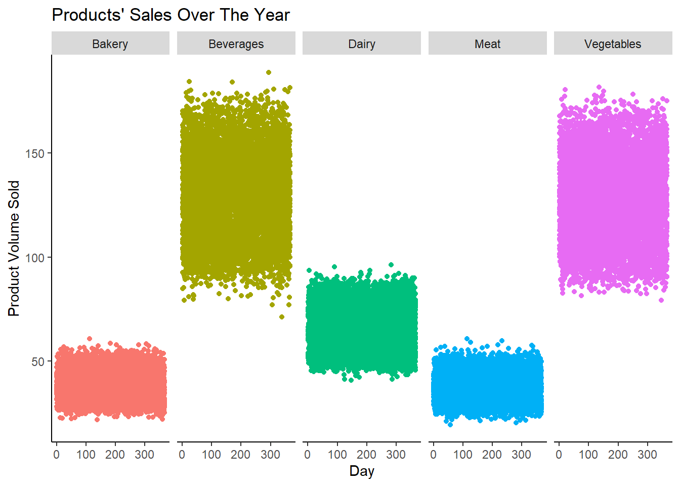
From the above chart, we can say that all products maintained respective sales pattern across the year. Vegetables & Beverages are the best sellers while Bakery and Meat are least sold products around the year.
final_restaurant_data |>
  mutate(Waste = Received_Order_Volume - Sold_Order_Volume) |>
  ggplot(aes(x = Received_Order_Volume, y = Waste, color = Product_Category)) +
  geom_point() +
  labs(
    title = "Received vs Waste by Product Category",
    x = "Received Order Volume",
    y = "Waste Volume"
  ) +
  theme_minimal() +
  theme(
    panel.grid.major = element_blank(),
    panel.grid.minor = element_blank(),
    panel.background = element_blank(),
    plot.background = element_blank(),
    axis.line = element_line(color = "black")
  )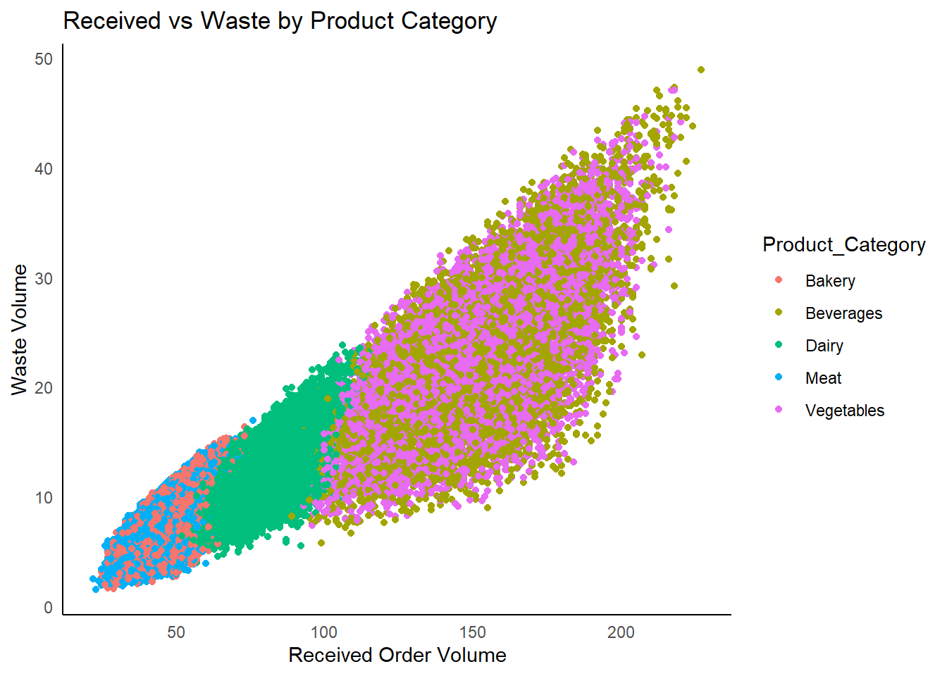
It is evident from the above graph that wastage is exponential with respect to the volume received.
final_restaurant_data |>
  mutate(Waste_Volume = Received_Order_Volume - Sold_Order_Volume) |>
  ggplot(aes(x = factor(Restaurant))) +
  geom_col(aes(y = Received_Order_Volume), fill = "red") +
  geom_col(aes(y = Sold_Order_Volume), fill = "green") +
  labs(
    x = "Restaurant",
    y = "Volume of Orders"
  ) +
  theme_minimal() +
  theme(
    panel.grid.major = element_blank(),
    panel.grid.minor = element_blank(),
    panel.background = element_blank(),
    plot.background = element_blank(),
    axis.line = element_line(color = "black")
  )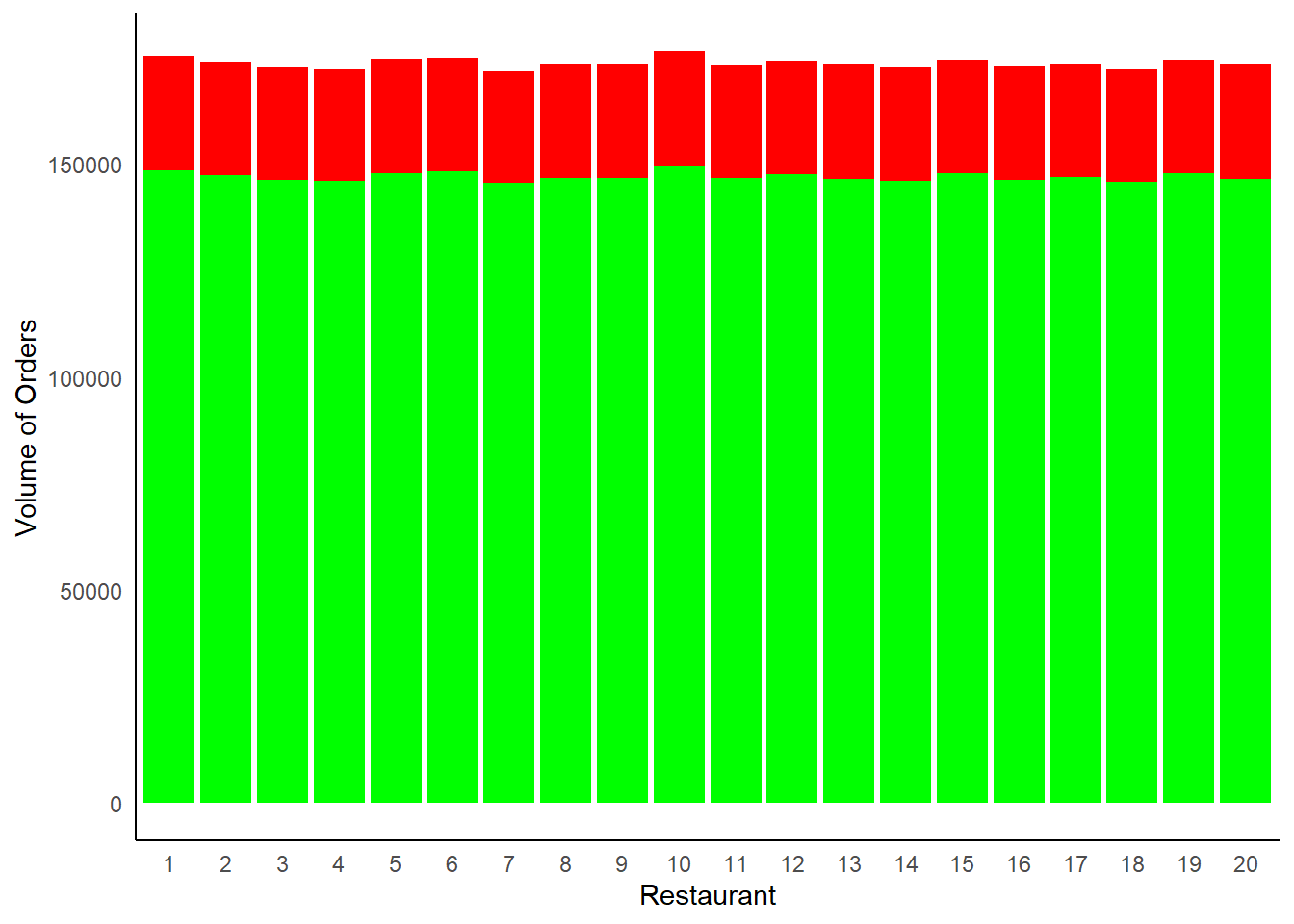
From the above chart, the red color length represents the wastage at each restaurant and green represent the units sold.
final_restaurant_data |>
  mutate(Waste = Received_Order_Volume - Sold_Order_Volume) |>
  ggplot(aes(x = Product_Category, y = Waste, fill = Product_Category)) +
  geom_bar(stat = "identity") +
  labs(
    title = "Waste by Product Category",
    x = "Product Category",
    y = "Waste Volume"
  ) +
  theme_minimal() +
  theme(
    axis.text.x = element_text(angle = 0),
    panel.grid.major = element_blank(),
    panel.grid.minor = element_blank(),
    panel.background = element_blank(),
    plot.background = element_blank(),
    axis.line = element_line(color = "black"),
    legend.position = "none"
  )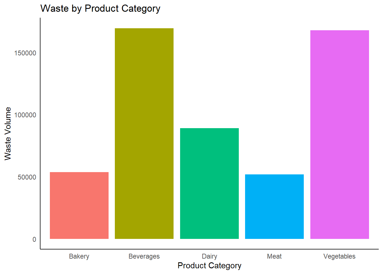
vegetables and beverages wastage is more than average volume wastage.
Given the configuration of 3-echelon supply chain, I assumed that received volume at each layer is something ordered by that layer from previous layer.
supplier_data <- read_csv("files/Daily_Supplier_Production_Shipment_Data.csv")
dc_data <- read_csv("files/Daily_DC_Shipping_and_Received_Data.csv")
Let us first understand a bit about the datasets.
supplier_data# A tibble: 527,913 × 6
Day Supplier Distribution_Center Product_Category Shipped_Volume
<dbl> <chr> <chr> <chr> <dbl>
1 0 S27 A Bakery 5
2 0 S28 A Bakery 4
3 0 S29 A Bakery 4
4 0 S30 A Bakery 2
5 0 S27 C Bakery 4
6 0 S28 C Bakery 9
7 0 S29 C Bakery 7
8 0 S30 C Bakery 4
9 0 S27 E Bakery 5
10 0 S28 E Bakery 4
# ℹ 527,903 more rows
# ℹ 1 more variable: Production_Volume <dbl>dc_data# A tibble: 95,160 × 6
Day Distribution_Center Restaurant Product_Category Shipped_Volume
<dbl> <chr> <dbl> <chr> <dbl>
1 0 A 1 Bakery 14
2 0 C 1 Bakery 23
3 0 E 1 Bakery 13
4 0 A 1 Beverages 60
5 0 C 1 Beverages 47
6 0 E 1 Beverages 71
7 0 C 1 Dairy 49
8 0 E 1 Dairy 38
9 0 A 1 Meat 20
10 0 C 1 Meat 13
# ℹ 95,150 more rows
# ℹ 1 more variable: Received_Volume <dbl>I identified that there was limited relationship in the given data among all three layers in the supply chain.
Hence, I assumed that, in a supply chain, it doesn’t matter which specific product from which Supplier reaches to which specific Restaurant. A Distribution Center accumulates each prodcut and delivers to restaurants accordingly.
This led me to exclude the continuous relation from Supplier ID > Distribution Center > Restaurant
supplier_agg <- supplier_data |> select(-2,-3) |> group_by(Day,Product_Category) |>
  summarize(overall_supplier_produced = sum(Production_Volume),
  overall_supplier_shipped = sum(Shipped_Volume))
`summarise()` has grouped output by 'Day'. You can override using the `.groups`
argument.supplier_agg# A tibble: 1,830 × 4
# Groups: Day [366]
Day Product_Category overall_supplier_produced overall_supplier_shipped
<dbl> <chr> <dbl> <dbl>
1 0 Bakery 1226 990
2 0 Beverages 3356 3099
3 0 Dairy 1860 1580
4 0 Meat 1236 947
5 0 Vegetables 3453 3052
6 1 Bakery 1210 974
7 1 Beverages 3597 3322
8 1 Dairy 1971 1692
9 1 Meat 1242 952
10 1 Vegetables 3580 3179
# ℹ 1,820 more rowsdc_agg <- dc_data |> select(-2,-3) |> group_by(Day,Product_Category) |>
summarize(overall_dc_received = sum(Received_Volume),
overall_dc_shipped = sum(Shipped_Volume))`summarise()` has grouped output by 'Day'. You can override using the `.groups`
argument.dc_agg# A tibble: 1,830 × 4
# Groups: Day [366]
Day Product_Category overall_dc_received overall_dc_shipped
<dbl> <chr> <dbl> <dbl>
1 0 Bakery 990 930
2 0 Beverages 3099 2970
3 0 Dairy 1580 1511
4 0 Meat 947 887
5 0 Vegetables 3052 2936
6 1 Bakery 974 910
7 1 Beverages 3322 3179
8 1 Dairy 1692 1614
9 1 Meat 952 890
10 1 Vegetables 3179 3062
# ℹ 1,820 more rowssupplier_dc_joined <- supplier_agg |>
left_join(dc_agg, by = c("Day", "Product_Category")) |> select(-4)
supplier_dc_joined# A tibble: 1,830 × 5
# Groups: Day [366]
Day Product_Category overall_supplier_produced overall_dc_received
<dbl> <chr> <dbl> <dbl>
1 0 Bakery 1226 990
2 0 Beverages 3356 3099
3 0 Dairy 1860 1580
4 0 Meat 1236 947
5 0 Vegetables 3453 3052
6 1 Bakery 1210 974
7 1 Beverages 3597 3322
8 1 Dairy 1971 1692
9 1 Meat 1242 952
10 1 Vegetables 3580 3179
# ℹ 1,820 more rows
# ℹ 1 more variable: overall_dc_shipped <dbl>let’s take the final_restaurant_data we create earlier as part of our analysis and make use of it join it to our supplier dc joined data.
dc_restaurant_joined <- final_restaurant_data |>
                      select(-2) |>
                      group_by(Day,Product_Category)|>
                      summarise(overall_rest_received = sum(Received_Order_Volume),
                      overall_rest_sold = sum(Sold_Order_Volume)) |>
                      mutate(Original_Day = Day,
                              Day = Day - 1)
`summarise()` has grouped output by 'Day'. You can override using the `.groups`
argument.dc_restaurant_joined# A tibble: 1,830 × 5
# Groups: Day [366]
Day Product_Category overall_rest_received overall_rest_sold Original_Day
<dbl> <chr> <dbl> <dbl> <dbl>
1 0 Bakery 930 773. 1
2 0 Beverages 2970 2555. 1
3 0 Dairy 1511 1277. 1
4 0 Meat 887 746. 1
5 0 Vegetables 2936 2505. 1
6 1 Bakery 910 764. 2
7 1 Beverages 3179 2696. 2
8 1 Dairy 1614 1363. 2
9 1 Meat 890 752. 2
10 1 Vegetables 3062 2635. 2
# ℹ 1,820 more rowssupplier_dc_restaurant <- supplier_dc_joined |>
left_join(dc_restaurant_joined,
by = c("Day","Product_Category")) |> select(-5)
supplier_dc_restaurant# A tibble: 1,830 × 7
# Groups: Day [366]
Day Product_Category overall_supplier_produced overall_dc_received
<dbl> <chr> <dbl> <dbl>
1 0 Bakery 1226 990
2 0 Beverages 3356 3099
3 0 Dairy 1860 1580
4 0 Meat 1236 947
5 0 Vegetables 3453 3052
6 1 Bakery 1210 974
7 1 Beverages 3597 3322
8 1 Dairy 1971 1692
9 1 Meat 1242 952
10 1 Vegetables 3580 3179
# ℹ 1,820 more rows
# ℹ 3 more variables: overall_rest_received <dbl>, overall_rest_sold <dbl>,
# Original_Day <dbl>In order to make the visulizations better understandable, I haven broken the 365 days into months, assuming that this data is an year’s data. So you might be seeing values like January etc., in upcoming visualizations.
df <- supplier_dc_restaurant
df <- df |>
  mutate(month = case_when(
    Day <= 30 ~ "January",
    Day <= 58 ~ "February",
    Day <= 89 ~ "March",
    Day <= 119 ~ "April",
    Day <= 150 ~ "May",
    Day <= 180 ~ "June",
    Day <= 211 ~ "July",
    Day <= 242 ~ "August",
    Day <= 272 ~ "September",
    Day <= 303 ~ "October",
    Day <= 333 ~ "November",
    TRUE ~ "December"
  )) |> relocate(month)

# Create a 'date' column using the base date (e.g., "2024-01-01") and adding the 'Day' column
df <- df |>
  mutate(date = as.Date("2024-01-01") + days(Day))

# Convert to xts objects using the 'date' column
supplier_produced <- xts(x = df$overall_supplier_produced, order.by = df$date)
dc_received <- xts(x = df$overall_dc_received, order.by = df$date)
restaurant_received <- xts(x = df$overall_rest_received, order.by = df$date)
restaurant_sold <- xts(x = df$overall_rest_sold, order.by = df$date)

# Combine all four series into one xts object for plotting
combined_data <- cbind(supplier_produced, dc_received, restaurant_received, restaurant_sold)

# Create the interactive plot using dygraphs
p <- dygraph(combined_data, main = "Comparison of Supplier, DC, and Restaurant Data") |>
  dyOptions(labelsUTC = TRUE, fillGraph = TRUE, fillAlpha = 0.1, drawGrid = FALSE) |>
  dyRangeSelector() |>
  dyCrosshair(direction = "vertical") |>
  dyHighlight(highlightCircleSize = 5, highlightSeriesBackgroundAlpha = 0.2, hideOnMouseOut = FALSE) |>
  dyRoller(rollPeriod = 10) |>
  dySeries("supplier_produced", color = "#FF6347", label = "Supplier Produced") |>
  dySeries("dc_received", color = "#4682B4", label = "DC Received") |>
  dySeries("restaurant_received", color = "#32CD32", label = "Restaurant Received") |>
  dySeries("restaurant_sold", color = "#FFD700", label = "Restaurant Sold")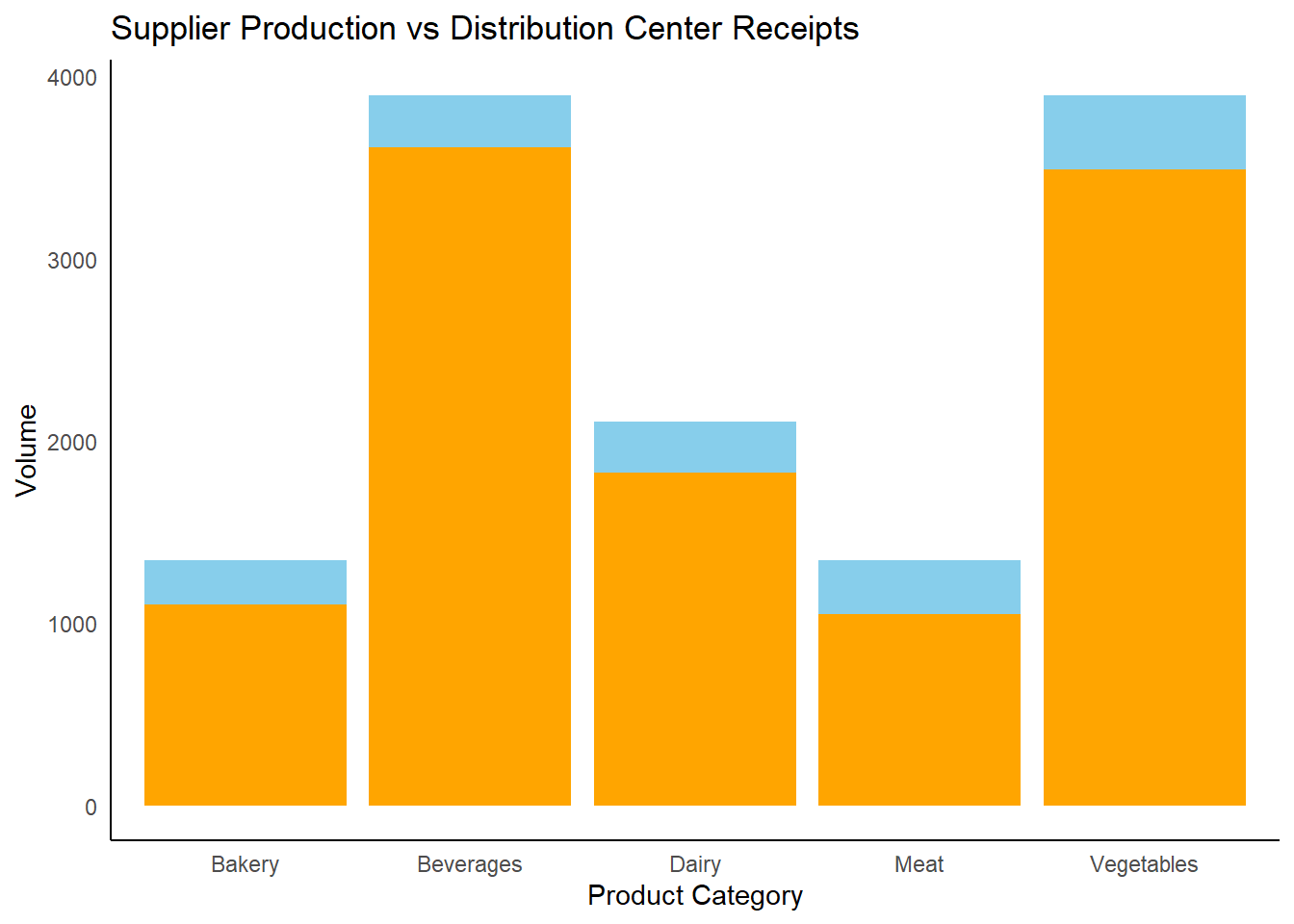
pggplot(supplier_dc_restaurant, aes(x = Product_Category)) +
geom_bar(aes(y = overall_supplier_produced, fill = "Supplier Produced"), stat = "identity", position = "dodge") +
geom_bar(aes(y = overall_dc_received, fill = "DC Received"), stat = "identity", position = "dodge") +
labs(title = "Supplier Production vs Distribution Center Receipts", x = "Product Category", y = "Volume") +
scale_fill_manual(values = c("Supplier Produced" = "skyblue", "DC Received" = "orange")) +
theme_minimal() +
theme(
axis.text.x = element_text(angle = 0),
panel.grid.major = element_blank(),
panel.grid.minor = element_blank(),
panel.background = element_blank(),
plot.background = element_blank(),
axis.line = element_line(color = "black"),
legend.position = "none"
)
library(tidyr)
library(ggplot2)

# Reshaping the data to long format for heatmap visualization
heatmap_data <- supplier_dc_restaurant |>
  pivot_longer(cols = c("overall_supplier_produced", "overall_dc_received"),
               names_to = "Stage", values_to = "Volume")

ggplot(heatmap_data, aes(x = Product_Category, y = Stage, fill = Volume)) +
  geom_tile() +
  scale_fill_gradient(low = "white", high = "blue") +
  labs(title = "Supplier Production vs Distribution Center Receipts Heatmap",
       x = "Product Category", y = "Stage") +
  theme_minimal() +
  theme(axis.text.x = element_text(angle = 45, hjust = 1))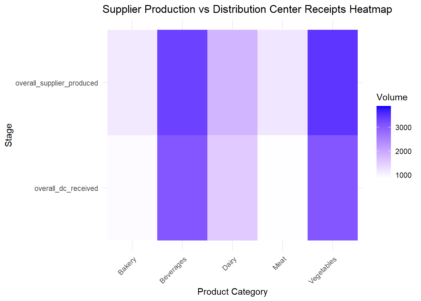
In this section, we clean the dataset to in order to understand the supply chain flow. For this I am trying to get the count of connections from each layer of the chain.
network1 <- supplier_data |> ungroup() |> select(2,3) |> distinct()
network2 <- dc_data |> ungroup() |> select(2,3) |> distinct()

s1 <- network1 |> group_by(Supplier) |> summarise(dc_count = n())


dc1 <- network1 |> group_by(Distribution_Center) |> summarise(supplier_count = n())
dc2 <- network2 |> group_by(Distribution_Center) |> summarise(restaurant_count = n())

r1 <- network2 |> group_by(Restaurant) |> summarise(dc_count = n())
dc_network <- dc1 |> left_join(dc2, by= "Distribution_Center" )s1# A tibble: 30 × 2
Supplier dc_count
<chr> <int>
1 S1 5
2 S10 3
3 S11 3
4 S12 3
5 S13 3
6 S14 3
7 S15 3
8 S16 3
9 S17 3
10 S18 3
# ℹ 20 more rowsdc_network# A tibble: 5 × 3
Distribution_Center supplier_count restaurant_count
<chr> <int> <int>
1 A 23 10
2 B 23 10
3 C 20 10
4 D 20 10
5 E 30 20r1# A tibble: 20 × 2
Restaurant dc_count
<dbl> <int>
1 1 3
2 2 3
3 3 3
4 4 3
5 5 3
6 6 3
7 7 3
8 8 3
9 9 3
10 10 3
11 11 3
12 12 3
13 13 3
14 14 3
15 15 3
16 16 3
17 17 3
18 18 3
19 19 3
20 20 3Now that we are done with pre processing let’s import these files into Tableau to take the visualizations to next level. You can access the Dashboard here:
Venkata's Tableau Dashboard URL